Artificial Neural Networks and Machine Learning

Seen from the outside, an artificial neural network is a program run by a computer. Its peculiarity compared to other programs is the ability to learn the relationships between the input data and the output data (the results), this is obtained through a basic logical structure that does not change as the data and relationships vary, but it adapts to them.
The name neural network comes from the comparison with that of our brain. Its structure provides a series of points, called nodes, connected to each other, which receive a numerical value from other nodes, increase or decrease it and return the result to new nodes. Similarly, neurons in our brain receive an electrical impulse from a series of neurons and can retransmit or not this electrical impulse to other neurons. After this explanation, a neuron doesn’t seem like a very intelligent object. It gets small shocks and all it does is relay them or not to other neurons. How can all this current spinning in our head turn into such complex actions we can perform? The secret lies in the quantity. For example, if we had 100 neurons, not only we would not be very intelligent, but, considering that we are made, they would not even be enough to keep us alive (however there are animals that do not have any neurons, such as sponges). What if we have 1000? It wouldn’t make much difference, just think that a jellyfish has about 6000 and belongs to the category of fauna with the smallest brain capacity. A mouse already has around 70 million and we humans reach 86 billion. But how does quantity transform such a basic and banal process into the amazing abilities we possess? To get to the answer, let’s analyze an artificial network.
The artificial neural network
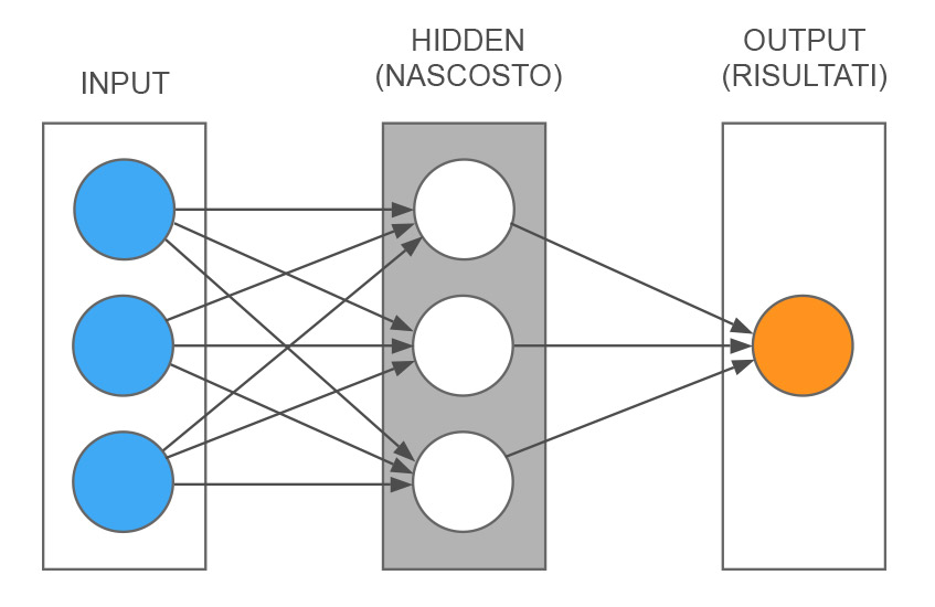
Diagram of a simplified artificial neural network
Let’s start by schematizing an example of a very simple neural network to understand its mechanism in detail. As you can see in the figure, we have three levels. One of the inputs, where, in this case, there are three nodes (blue circles), these three nodes represent three input information. A central level, called hidden because it does not communicate directly with the outside (white circles). And a layer on the right that represents the results, in this case, made by a single node (orange circle). The gray lines show the connections between the various nodes. The simplest way to explain how it works is with an example.
An example of a weather forecast
We use an extremely simplified weather forecast model. Suppose we want to forecast if it will rain or not an hour from now, based on three simple factors: 1) The number of clouds in the sky, 2) The wind speed, 3) The possible amount of rain at this moment. Our three inputs will be decimal numbers that can go from 0 to 1. For example, for the first factor, the number of clouds, we will have a 0 if there is no cloud in the sky, a 0.5 if the clouded areas and the clear ones are equivalent, up to 1 in the case in which the whole sky is covered with clouds. So we can see our cloud value as the percentage of the sky covered by clouds. We will do the same for the other two factors, i.e. the wind factor, which will be 0 in case of total absence up to 1 in case of maximum speed (the maximum speed will be defined a priori depending on the geographical area where we are making the forecast). Finally, we assign the value of the amount of rain, 0 in case of total absence up to 1 for the maximum intensity. To keep the example as simple as possible we have only one result and we call it raining.
The hidden level
Now that we have decided which are the inputs and outputs of our neural network, we can proceed to explain what this elusive intermediate level does. As you can see from the figure, each of the white dots (that represent neurons) receives all three inputs. So each of these nodes receives three numbers between 0 and 1. The first thing it does is assign a “weight” to each of these three values. This means that it defines a percentage for each of the inputs. Then it calculates these percentages and adds them. Let’s see an example.
Let’s take these three inputs: Clouds = 0.8; Wind = 0.1; Rain = 0.3. We are in a very cloudy sky, with very little wind and a little rain. The first node decides to give the cloudiness a weight of 35%, the wind a weight of 52% and the rain a weight of 2%. So the input values of this node will become 0.8 x 0.35 = 0.28; 0.1 x 0.52 = 0.052; 0.3 x 0.02 = 0.006. After doing these calculations, the node adds up the three results: 0.28 + 0.052 + 0.006 = 0.338. I guess you are asking yourself two questions, where did it take those percentages to calculate the weight of each input? Why does it do this? We begin to answer the first, for the second the answer will come later. These percentages are random. Well, you will say, everything already seemed not intelligent before, now that it makes up numbers it just seems pointless. In reality, we can say that at this point in the process, our system is ignorant, because it has not yet used intelligence to learn, but it will.
The next step is to define a threshold, that is a minimum value beyond which this information will go forward or not. In this case, for example, we can define that if the result of the calculation of a node exceeds 1.5 then the signal is transmitted over, otherwise it stops there. Also for this value, we don’t know a priori which is the correct one for each node, so we could set any number. However, in this case, I introduced the result of my reasoning into the neural network, choosing the average of the sum of the inputs. In our example, the sum of the three inputs can range from 0 (when they are all zero) to 3 (when they are all one). I did this to show how it is possible to start a neural network with parameters that already make sense, therefore knowledge and reasoning come from outside the neural network. The advantage of doing this is simply decreasing the time the network will take to get to the results, but it is not at all a necessary thing. To mathematically obtain the continuation or not of the information, we introduce a function that generates the value 0 if the result of the previous calculation is less than 1.5 or generates a 1 if the result is greater than this threshold. Then a 0 or a 1 will exit the node.
The results of artificial thinking
Now we are at the last level, that of the result. Each central node is connected to the result node, which we called raining. This node receives a 0 or a 1 from all the central nodes, exactly as before, it applies a weight to each incoming value and has a threshold value, under which the same mathematical function will generate a 0, and above it will generate a 1. So nothing different than the previous level. We were at the point when the first node of the central level calculated the value 0.338, which is less than 1.5, so it sent a 0 to the result node. Therefore the result node received a 0 from the first central node. Let’s say it applies to it a weight of 71%, so it gets 0 x 0.71 = 0. Similarly, it received the values from the other two central nodes, so we assume the other values with their weight and do the same sum we did for the central nodes: 0 x 0.71 + 1 x 0.27 + 1 x 0.95 = 1.22. In this case, without doing any reasoning, we decide that the threshold of this node is 2, therefore being 1.22 less than 2 our mathematical function will generate a 0. What does it mean that the node of the result raining is equal to zero? We decide what it means, and we say that if the value is 0 then it will not rain in an hour, whereas, if it is 1 it means that it will rain in an hour. In this example, our neural network told us that it will not rain. If the process ended here it would have the same value as tossing a coin and deciding that heads mean it will rain and tails no, so now we need to make our neural network capable of learning.
Machine learning
To allow the neural network to learn what relationships there are between the input information and the results, we need real data. In our example we have to collect data on cloud coverage, wind speed and rain intensity for a certain period of time. With this information, we have both the inputs and the results, because, if we collect the data every hour, we know that the intensity of rain at a certain time is what I should have predicted an hour earlier, so I am going to correlate it to the three parameters of the previous hour. In our very simple case, the result is not even intensity, but simply the presence or absence of rain. Once I have a good amount of data (obviously the larger it is, the more reliable the predictions will be), I apply what is called the error back-propagation to the neural network.
In other words, it is nothing more than a kind of trial-and-error learning. When the network works on the historical data series, it can make a comparison between the results obtained and the real data. In general, there will be a difference between the two values, therefore an error. The purpose of learning is the same as for a human being, to stop making mistakes, or better, to reduce them as much as possible. In our very simplified example, the neural network could calculate a 0 when the correct result had to be a 1, so no rain when it actually rained (and vice versa). Let’s assume that out of 100 real measurements, in 30 cases the result is correct, while in the remaining 70 it is wrong. To reduce the percentage of errors, the neural network can modify the parameters we saw earlier: the weight of the inputs and the threshold that determines whether the output of the node is 0 or 1.
How to optimise the parameters
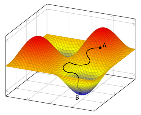
Example of a function that represents the error of the result in relation to weights and thresholds, that is, the parameters that the neural network can vary.
A first hypothesis is to continue modifying randomly these values for each node until the error drops below a certain level that we consider acceptable. By doing so we would have a neural network that has learned the correlations between inputs and results. This system could perhaps work for our example composed of a handful of neurons, but think of a network made up of hundreds of thousands of nodes, surely a lifetime would not be enough to see the result, most probably it would go beyond the duration of the universe from its birth to now. Then we have to think about smarter ways to find the correct parameters. We can use a mathematical function that contains our parameters and represents our error, and what we have to do is find where it is minimum (and therefore where the error is minimum). In the image we see an example of an error function in two variables: a curved surface with maxima and minima (peaks and troughs). What we need to do is change our parameters to get to the bottom of the lowest trough. In this case, we assume that with the initial parameters, which cause an error of 70%, we are in point A. We must find a way that, in the shortest possible time, takes us to point B, where we find the parameters that give the minimum error and make our network capable of making this weather forecast. To obtain this, there are very effective mathematical methods, such as stochastic gradient descent. Understanding these methods implies a substantial mathematical study and the purpose of this post is to explain the general concept. I have put the Wikipedia link for the more curious and stubborn readers who wish to delve into the subject.
More complex networks
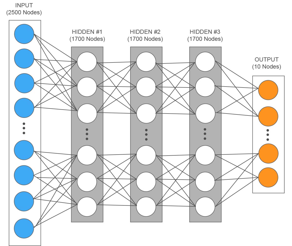
Example of a network for the recognition of handwritten digits with a resolution of 50×50 pixels, each input represents a pixel.
Now our network has the correct parameters, so it has learned what the relationships between inputs and results are and is able to predict if it will rain in an hour with a contained error. This example is extremely simplified, in reality neural networks can handle a much higher number of inputs and the results can also consist of multiple neurons. The intermediate level can be composed of several levels, where each one does a part of the work and passes the partial result to the next level. Let’s take the example of a network that recognises handwritten numbers, where a single digit is an image consisting of 50 x 50 pixels, so it would have 50 x 50 = 2500 input values. Let’s assume three intermediate levels, each composed of 1700 neurons and 10 for the results (the ten possible digits from 0 to 9), would be 5110 neurons in total. Now we can calculate how many parameters there would be to be optimised with each neuron of a level connected to all neurons of the previous level: 1700 x 2500 (weights) + 1700 (thresholds) + 1700 x 1700 (weights) + 1700 (thresholds) + 1700 x 1700 (weights) + 1700 (thresholds) + 10 x 1700 (weights) + 10 (thresholds) = approximately 10 million parameters. A final point to note is that in addition to the increase of neurons and connections, artificial neural networks can work together with other algorithms, creating a more efficient hybrid system.
Why the size makes the difference
Let’s go back to the question we asked ourselves at the beginning. Now that we have an idea of the operating principle of a neural network, we can also understand why a greater number of neurons implies greater skills. Actually, we should also talk about the number of connections. Thanks to them it is possible to have very complex mixes of inputs and therefore the possibility of manipulating in a more refined way what enters a neuron. We must think that a neuron does an extremely simple operation, so if we want to obtain a complex capacity, we must divide it into a certain number of elementary operations, which, combined together, will be able to give the result. If I have many input values, as in the example of the image of the handwritten number, in order to manage them all and not lose information, the number of neurons must be high. Let’s try to exaggerate and put only one neuron in the intermediate level, it will receive altogether the information of the 2500 pixels. It will only be able to vary their weights before adding them all, in this way, however, it will only have a value that will be an average of all the individual values, which says absolutely nothing about the image. If, on the other hand, we have more neurons, the first will only be able to give more weight to certain pixels and send that information forward, the second to others, and so on. In this way, the information is not lost and is processed more and more at each step up to the last level, that of results, where the neuron corresponding to the recognized figure will release the value 1. This division of tasks between neurons is obtained with the learning phase and the relative optimisation of the parameters as we have seen in the previous paragraph.
Lack of intelligence or learning?
Let’s give an example of the human brain. You went abroad, to a country whose language you absolutely do not know. A person approaches you and speaks to you in this language, your brain processes all the sound information received from the ears, each neuron is activated or not by the set of electrical impulses and, depending on the threshold, sends information or not to the following neurons. and so on until the results. But the results won’t make sense, they’ll just be a jumble of unknown sounds, even though your brain has done the same job it always does. The difference compared to when we listen to a dialogue in a known language is that in this case the learning part is missing, where all the parameters are set to process the inputs and give a useful result. Also in this case all the information coming from the person who spoke to you was lost, but unlike the example of the single neuron, that could not process the information of 2500 pixels by itself (lack of intelligence), in this situation, the number of neurons would have been enough, but the previous learning phase was missing.
In the next post, we will talk about what concrete results can be obtained with an artificial neural network and its main practical applications with the enormous benefits it brings.

